8 Must Know Spreadsheet Tips for Managing Your Product Information

When it comes to managing product information, spreadsheets are a trusted companion for countless ecommerce businesses. Their versatility and widespread usage make them a go-to tool for organizing and managing product data. 

In this blog post, we’ll discuss eight must-know spreadsheet tips that you can use to improve your product data management. While we delve into these tips, keep in mind that, although spreadsheets are an exceptional starting point, a dedicated Product Information Management (PIM) system can always help take your data management to the next level. 

For now, let’s explore the world of spreadsheets and discover how these tips can optimize your product data management process.

1. Keep errors at bay with data validation

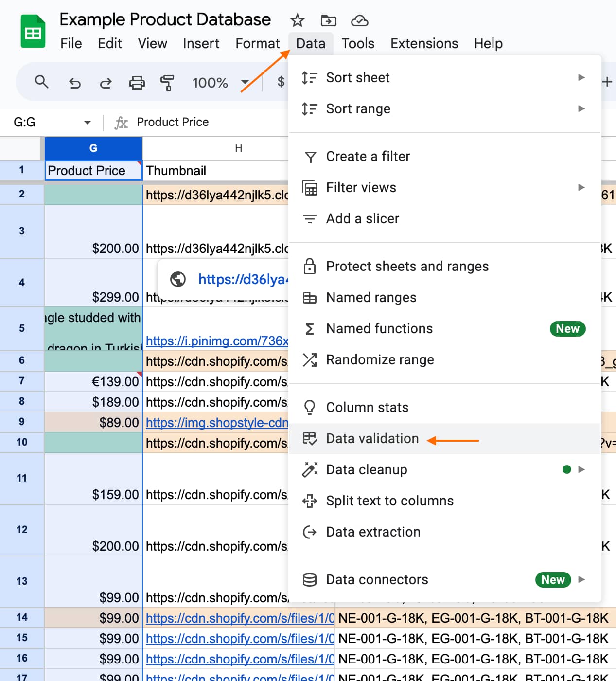
Tip number 1 is using ‘Data Validation’ to make sure that your data adheres to the specific criteria that you set. Data validation is your first line of defense against data entry errors. Using it ensures consistency and accuracy throughout your product information. 

How to do it

Select the cell or cell range you want to validate, go to the “Data” tab, and click “Data Validation.” From there, you’ll need to define your criteria. You may want to check for specific values, such as date ranges or specific text.  

How to do it

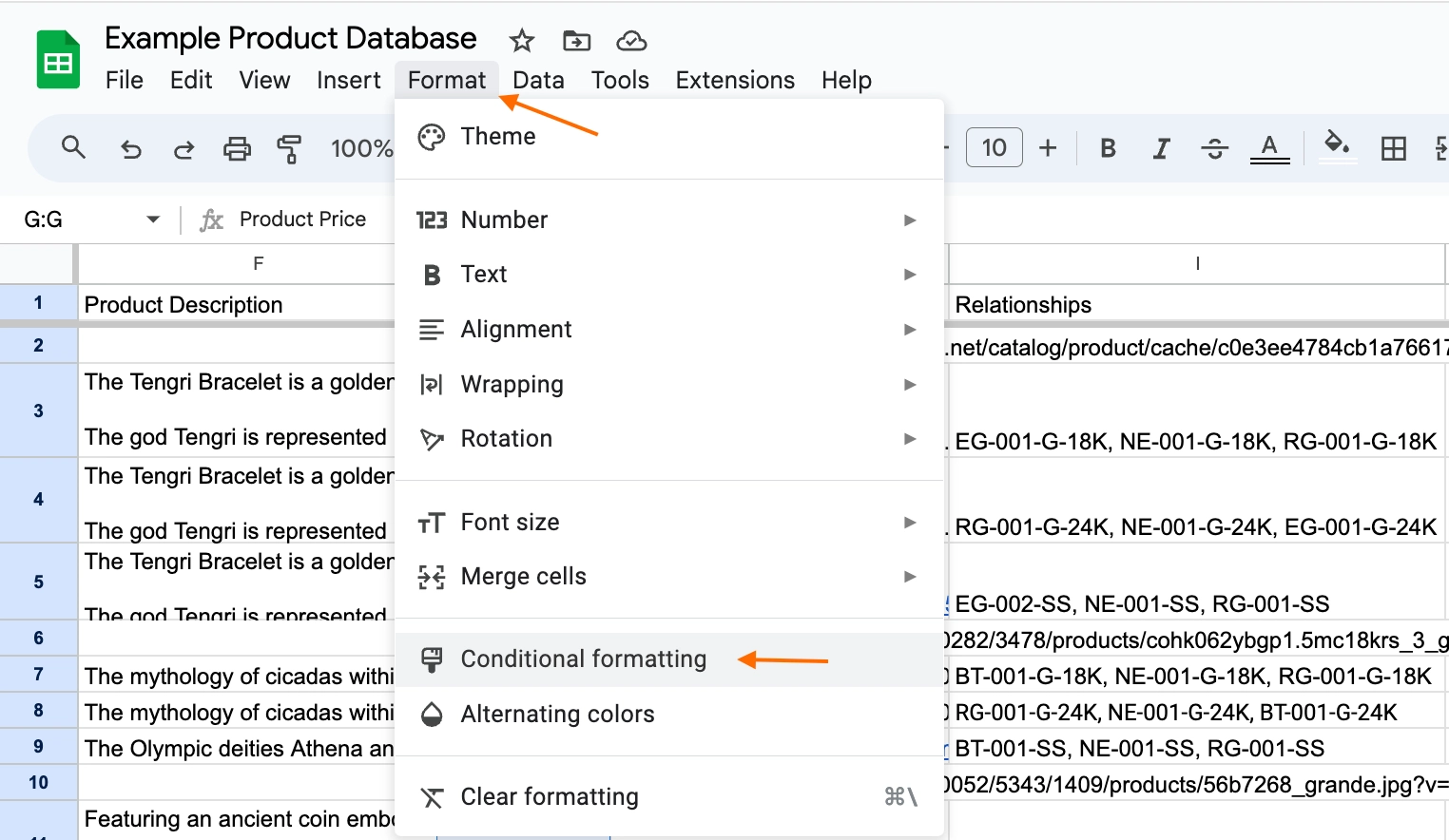
Select the range you want to analyze, go to the “Format” tab, and click “Conditional Formatting.” Then, you can select the rule and formatting options you wish to apply.

3. Use pivot tables to make data analysis simple

When dealing with vast amounts of data, PivotTables are your go-to for data summarization. They offer a quick way to derive valuable insights from extensive datasets.

How to do it

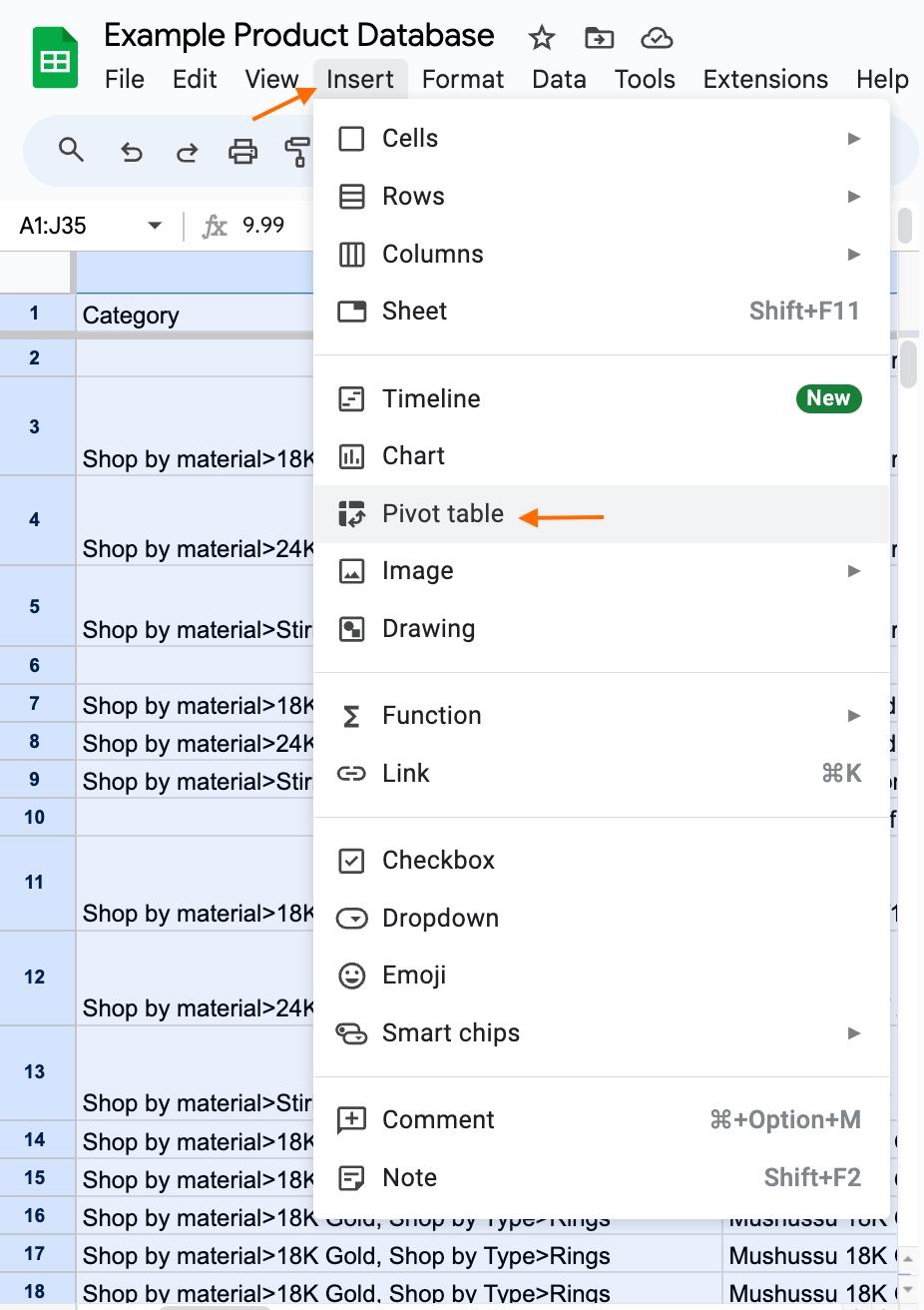
Select the data you want to analyze, go to the “Insert” tab, and click “PivotTable” and then “Create.” You can either add the table to your existing sheet or a new sheet, depending on your preferences. Google Sheets will recommend some data summaries for you, or you can customize your Pivot Table according to what information you want to see. You do this by choosing the fields and dragging them into the appropriate areas.

4. Refine your data with filters

Data filtering is your trusty sidekick for narrowing down your product list. Whether you need to view products in a specific price range or find out-of-stock items, data filtering is the way to simplify the process. With data filtering, you can view and manipulate specific subsets of your data.

How to do it 

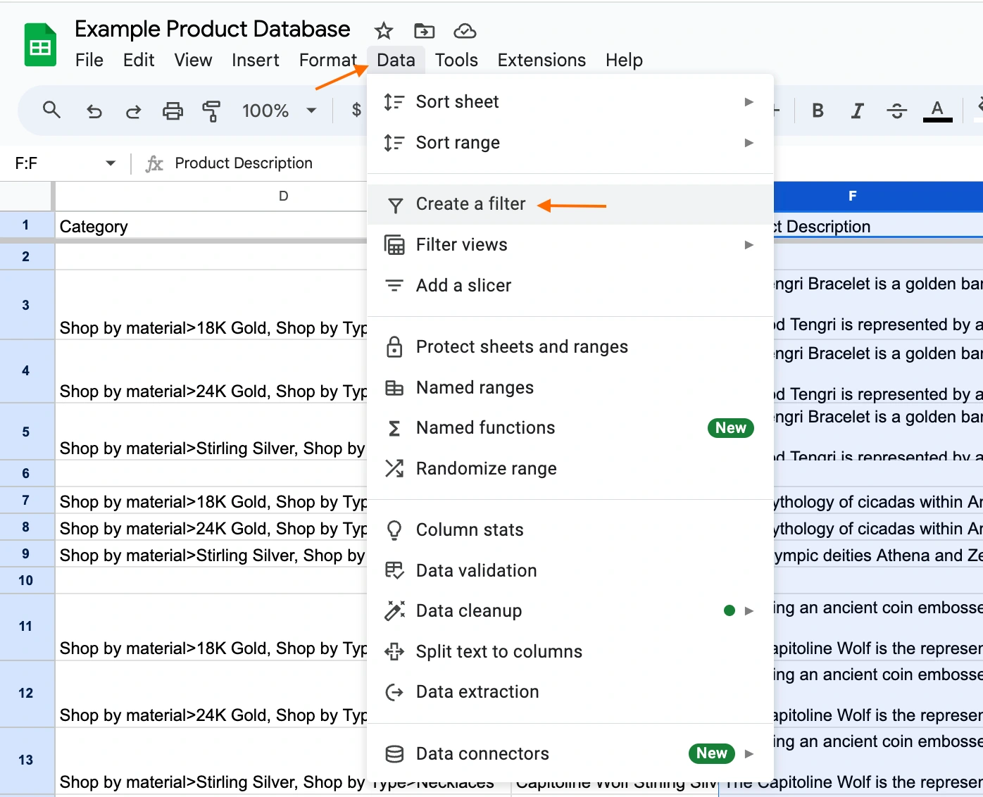
Select the data you want to apply a filter to, go to the “Data” tab, and click “Create a filter.” Then, use the drop-down arrows to filter data based on your criteria.

5. Simplify data presentation with custom views

Custom Views are your ticket to quickly accessing specific views of your product data depending on your needs. You can set up different views for different tasks, like marketing enrichment or product specifications. Custom Views enable you to save and switch between different settings for filtering, sorting, and other view options. 

How to do it

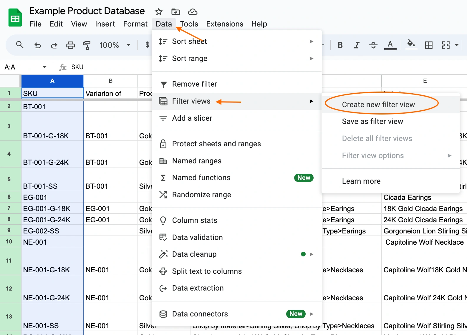
Select the columns you wish to work with, go to the “Data” tab, and click “Filter views,” and then “Create new filter view.” From here, you can make adjustments to your sheet, hide columns that aren’t relevant, or add other filters that are useful to you. Name your new filter and click the “X” when you’re ready to return to the regular sheet. Your view will be automatically saved and are viewable at any time. 

6. Seamlessly integrate your data with import and export

With Google Sheets, you can import and export data from various sources or other sheets. Google’s data import and export capabilities work well for integrating your product data with other systems. Making use of this feature simplifies data exchange, whether it’s with suppliers, ecommerce platforms, or other critical systems.

How to do it

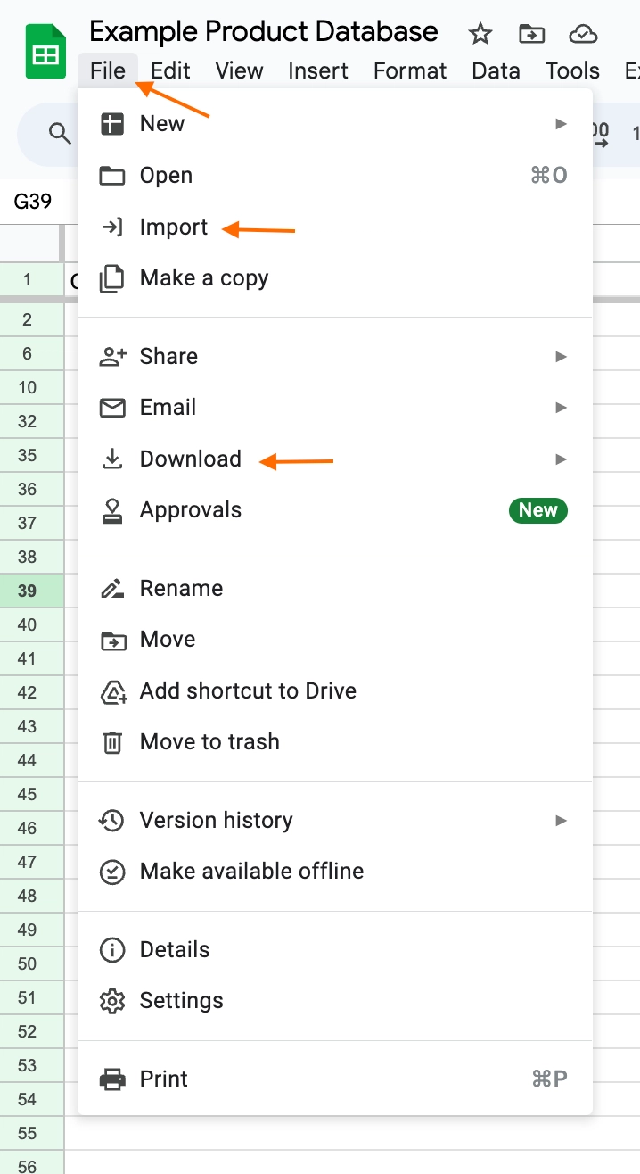
Go to the “File” tab, select “Import” to import data, and choose “Download” to export the data in the formats you need.

“How to merge product information from multiple sheets.”

7. Find data with ease using VLOOKUP

VLOOKUP is a lifesaver when you need to find specific information in a sea of data. VLOOKUP is a powerful function in Google Sheets (and other spreadsheet programs) that allows you to search for a specific value in a range or table and retrieve related information from that table. It’s commonly used for tasks like looking up specific product data or any other dataset where you need to find and retrieve particular details.

How to do it

The syntax for the VLOOKUP function is as follows: VLOOKUP(search_key, range, index, [is_sorted]

Let’s break down each part of this function:

• search_key: This is the value you want to look up. In your case, it could be a product name, ID, or any unique identifier.
• range: This is the range or table where you want to search for the search_key. Make sure the search_key is in the first column of this range and the data you want to retrieve is in subsequent columns. In a product data example, the range might include product names in the first column and product details (e.g., price, description) in adjacent columns.
• index: This is the column number (1, 2, 3, etc.) from which you want to retrieve data when a match is found. For example, if you want to get the price of a product, and the price is in the third column of your range, you would use 3 as the index.
• [is_sorted]: This is an optional argument. If you set it to TRUE (or omit it), VLOOKUP assumes that the first column of the range is sorted in ascending order. If set to FALSE, it assumes an exact match is required. For most product data scenarios, you would use FALSE because you want to find an exact match.

Here’s an example of how to use VLOOKUP in Google Sheets with product data:

Imagine you have two different sheets, one with your barcode and description and the other with your SKU and barcode, and you want to combine the data so that it’s all in one place and matching to each product correctly.

Your first sheet might look something like this: 

“Description and Barcode”

And your second sheet might look something like this: 

“SKU and Barcode”

In order to combine the two sets of data so that the SKU, Barcode and Description are all together for each product, you’d need to complete the following action;

=VLOOKUP(A2,’Description and Barcode’!A:B,2,False). 

• “A2”, is the search_key.
• “Description and Barcode’!A:B” is the range to search in
• “2” is the index to retrieve the description.
• “FALSE” indicates that you want an exact match.

The formula will return the matching descriptions for each product. 

8. Eliminate Duplicates

Keeping your data clean and organized is crucial. Eliminating duplicates helps to maintain data integrity by removing repeated entries so that your product information remains accurate.

How to do it

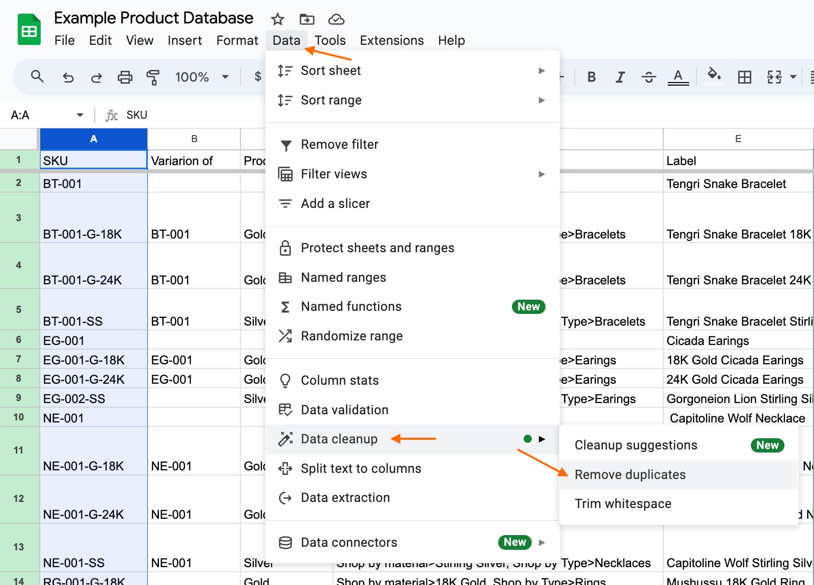
Choose the columns you wish to check for duplicates, go to the “Data” tab, and click “Data clean up,” followed by “Remove duplicate data.” Doing this will automatically delete any repeated data throughout your selected area.

Edit in bulk: With PIM, you can search, edit, and replace old data in just a few clicks. You simply use the bulk edit function to make changes to thousands of products simultaneously. 

While you apply these tips to your daily routine using spreadsheets, keep PIM in mind as the ultimate solution to master the art of product data management. PIM ensures data accuracy, consistency, and scalability, and it provides a user-friendly interface to help your product information management reach new heights.

To discover how PIM adopters are outperforming their competitors, grab your free copy of the ebook How PIM Adopters Outperform their Competition.